Demand forecasts often look good until you zoom in to the SKU level.
What looked stable on a high level and on paper quickly turns inconsistent in practice. Some products go out of stock, while others sit unsold.
This gap is hard to ignore. It shows that “good enough” forecasting at an aggregated level doesn’t translate into accurate execution.
In this article, we will discuss what is SKU-level forecasting, what makes it challenging, how to correctly measure accuracy, and which technologies can help improve SKU-level demand forecasting accuracy in real-world conditions.
What is SKU-level Demand Forecasting?
SKU-level demand forecasting = predicting how much of each specific product you’ll sell.
Unlike category-level planning, it focuses on individual items – by size, flavor, format, or store.
This level of detail makes forecasting more realistic, but also harder to measure.
The Main SKU Demand Forecasting Analysis Metric
One of the most common ways to evaluate accuracy is the MAPE (Mean Absolute Percentage Error) metric. It shows how far sales forecasts deviate from actual sales, expressed as percentages.
MAPE = (1/number of periods) * Σ ((actual demand – forecast) / actual demand) * 100
In simple terms, MAPE tells you the average percentage error between what you predicted and what actually happened.
How to Read It
- 0% MAPE – perfect sales forecast
- 10% MAPE – forecasts are off by around 10% on average
- 30%+ MAPE – weak accuracy (common at SKU level)
The lower the MAPE, the better the SKU-level forecasting.
Types of SKU Forecasting Methods
| SKU Demand Forecasting Methods | |
| Method | When to use |
| Baseline forecasting | Demand is stable, and you have solid historical sales data per SKU |
| Demand driver model | Demand is influenced by promos, pricing, or external factors that you can track |
| Machine learning | You manage many SKUs, and multiple factors impact demand at once |
| Aggregate-and-distribute | SKU-level data is weak (new or low-volume products) |
Time-Series Approaches
In simple terms, you look at the past and assume a similar pattern will repeat in the future.
For instance, a brewing brand tracks sales of a specific SKU – say, a 330 ml beer can. They do some SKU analysis, and here’s what they see in the past:
- Sales increase every summer
- Drop during colder months
- Spike during weekends and holidays
Based on this pattern, the brand assumes:
- higher production and distribution volumes for summer
- lower volumes for winter
- additional stock before weekends and holiday periods
There are two ways this approach can be applied in practice: using only past sales (like in the example above), or considering additional factors beyond past sales.
1. Baseline demand model (no extra info)
Even this, the simplest and most logical approach, requires tons of data.
Businesses need some infrastructure to gather sales numbers weekly or even daily. By country, region, and channel.
In many companies, the data is scattered between spreadsheets and systems. Performing SKU demand forecasting under such conditions requires a lot of manual work.
Manual preparation slows down demand forecasting at the SKU level and introduces errors:
- missing weeks
- duplicated entries
- inconsistent products naming
| Where the baseline demand model works well | Where the baseline demand model breaks |
| Mature products | New product launches |
| Stable demand | Promotions |
| No major market changes | Competitor disruptions |
2. Demand driver model (Past sales + external factors)
In this case, you still use sales history but also add drivers – data on some external factors about each SKU.
For each SKU, you add data like:
- Promo calendar (discounts, bundles)
- Price changes by channel
- Marketing campaigns
- Weather (for seasonal categories)
- Sales team input (expected orders from key accounts)
Let’s say a beverage brand is doing SKU forecasting analysis for a 1L iced tea SKU.
What the historical data says:
- Average sales: 8,000 units per week
- Summer uplift: +25% → around 10,000 units
If they stop here, that’s their sales forecast.
What if they add real inputs for the next month:
- 15% discount in two key retail chains
- Feature in a national promo leaflet
- Heatwave expected in key regions
- Their sales team confirms a large order from a distributor
Now the forecast has changed. And demand will be, for example, closer to 13,000-14,000 units instead of 10,000.
| Where the demand driver model works, and where it breaks | ||
| Situation | Works well when… | Breaks when… |
| Data availability | You have consistent data on promos, pricing, and sales by SKU | External data is missing, inconsistent, or not linked to SKUs |
| Promotions | Promotions are planned and tracked (discounts, leaflets, bundles) | Promo data is incomplete or not reflected in historical sales |
| Market conditions | Demand is influenced by clear, measurable factors (weather, campaigns, pricing) | Demand shifts are driven by unpredictable events (e.g., sudden competitor moves) |
| Sales input | Sales team provides structured, realistic forecasts (e.g., confirmed orders) | Inputs are subjective or overly optimistic |
| SKU maturity | Established SKUs with enough history + driver data | New products with no reliable past or driver patterns |
| Scale | You can consistently apply the same inputs across markets and channels | Data varies by region or channel, making comparisons unreliable |
Machine Learning Forecasting Approach
Machine learning is a more advanced way of using the same inputs as a demand driver model. ML automatically learns complex relationships between them and updates forecasts as new data comes in.
Where to find an ML model
Machine learning models don’t exist as a standalone thing you download and run. You either use it through a tool or build it into your system. Here’s what happens behind the scenes:
- you connect your data (sales, promos, pricing)
- the system trains models automatically
- forecasts are generated per SKU
- updates happen regularly (daily/weekly)
From the user side, it looks simple: upload data – get forecast.
What SKU data ML models need as inputs:
- Past sales – baseline demand
- Promotions – expected uplift
- Price changes – elasticity effect
- Seasonality – recurring patterns
- External signals – weather, campaigns, market changes
For example, a brand takes one SKU – 1L iced tea:
- Base demand: 8,000 units
- Summer effect: +2,000
- Promo: +2,500
- Heatwave: +1,000
Final forecast: 13,500 units.
| Machine learning approach | |
| How it works | Learns complex relationships between multiple inputs automatically |
| Best for | Large SKU portfolios with many influencing factors |
| Limitation | Requires large, clean, and well-structured data |
Aggregate-and-Distribute Approach
The aggregate-and-distribute approach doesn’t forecast the SKU directly at all.
With the first two approaches we’ve discussed, each product is modeled individually. With aggregate-and-distribute, you first forecast at a higher level (category/brand), then split that forecast down to SKUs.
The approach is useful when SKU data is too weak (like for new or low-volume products), unlike time-series models, which require reliable SKU-level history.
| Aggregate-and-distribute approach | |
| How it works | Uses total demand and allocates it based on SKU share |
| Best for | New or low-volume SKUs with weak data |
| Limitation | Accuracy depends on the allocation logic |
For instance, a beverage brand launches a new flavored iced tea SKU. At the SKU level, there’s almost no usable data, just a few weeks of irregular sales. Not enough to identify any pattern.
Instead of forcing a forecast, the brand shifts the level of analysis – one of the practical SKU optimization strategies for demand forecasting. It estimates total demand for the iced tea category, say 120,000 units for the next month, using stable historical data across all SKUs.
That total is then distributed down. If the new SKU is expected to account for 10% of category sales, its forecast is 12,000 units.
Can Excel Deliver Accurate SKU Demand Forecasting?
Short answer: yes, but only up to a point.
Excel works well when a brand has a limited number of SKUs, clean data, and stable demand. In these cases, it’s enough to calculate trends, apply basic seasonality, and build straightforward forecasts.
Basically, it must be an extremely small brand in an environment that doesn’t change much.
For most brands, the reality is different, and Excel struggles to keep up.
As the number of SKUs grows, markets expand, and promotions become more frequent, Excel can’t handle the complexity.
6 Benefits of SKU-Level Demand Forecasting

Optimized Inventory Levels
You know how much of each SKU to produce and ship, not just at the category level.
Fast-moving items don’t run out, and slow movers don’t pile up in warehouses.
Lower Costs
You avoid producing units that won’t sell and discounting them later.
Logistics becomes more efficient because shipments are closer to actual demand. Cash is no longer tied up in inventory that sits idle.
Better Forecast Accuracy
Instead of averaging demand across products, you forecast each SKU based on its own behavior. This reduces errors caused by mixing fast and slow movers together.
Improved Customer Experience
Popular SKUs are less likely to be out of stock during peak demand. Retailers get a consistent supply, which improves shelf presence. This helps meet customer expectations, so end customers don’t switch brands due to availability issues.
Smarter Decision-Making
You can see which SKUs actually drive volume and profit. This helps with decisions like pricing, promotions, and product assortment. Underperforming products become visible and can be fixed or discontinued.
More Efficient Operations
Production, supply chain, and sales teams work with the same SKU-level plan.
Fewer last-minute changes are needed because demand is clearer upfront. Replenishment becomes more predictable and less reactive.
Teams spend less time fixing issues and more time executing plans.
Challenges of SKU Demand Forecasting
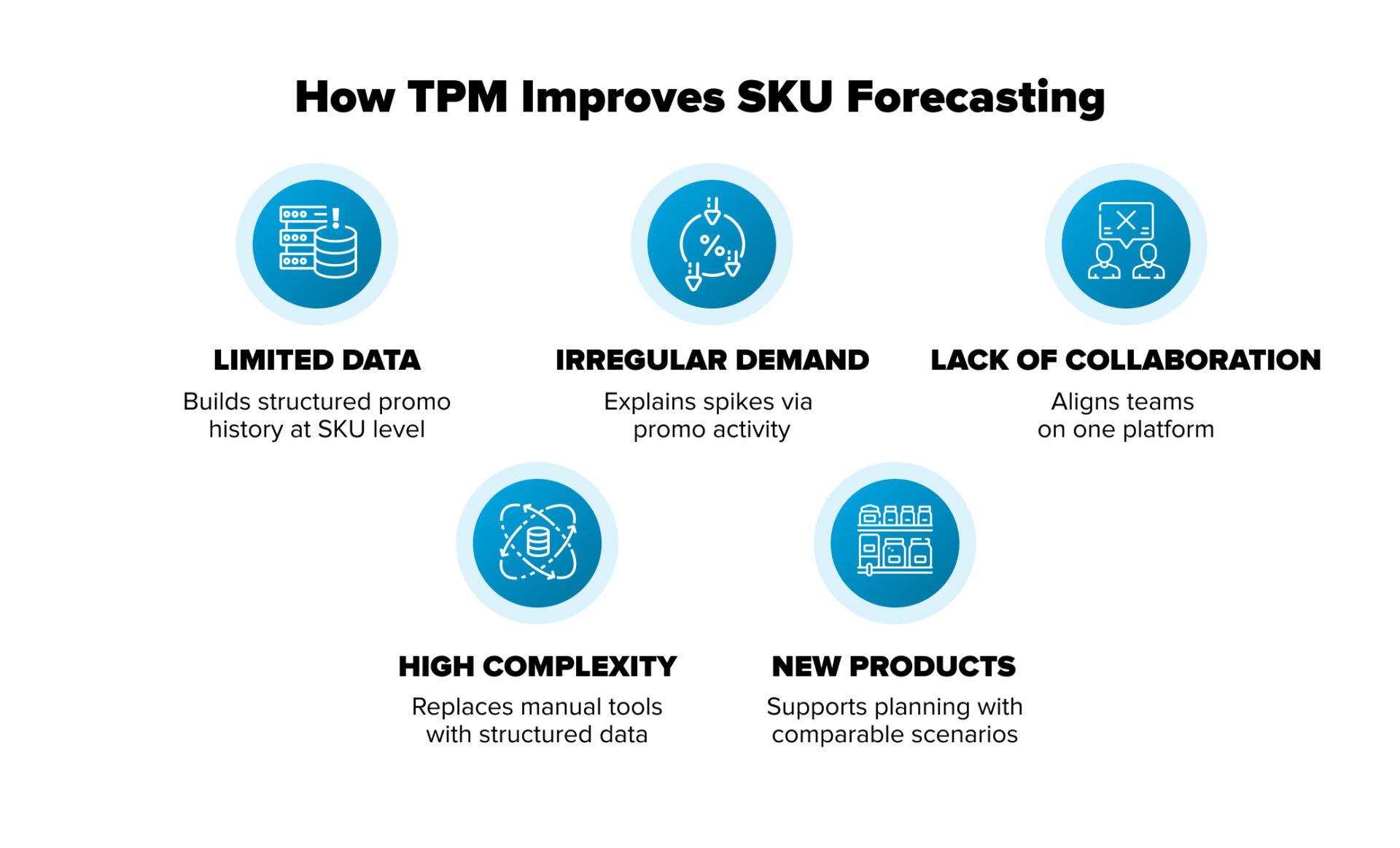
| What Makes SKU Demand Forecasting Difficult | |
| Limited Data Availability | Data is incomplete or scattered, so forecasts are built on weak foundations |
| Irregular Demand Patterns | Demand spikes (promos, seasonality) are misread as normal trends |
| Lack of Collaboration | Teams plan separately, leading to mismatched forecasts and stock issues |
| High Data Volume & Complexity | Too many SKUs and variables overwhelm manual tools and simple models |
| New Product Launches | No historical data, so forecasts rely on assumptions and often miss |
Limited Data Availability
Any sort of calculation (from basic statistics to advanced AI forecasting) needs historical records.
At the SKU level, this means consistently capturing sales, pricing, and promotional activity across markets and channels. In practice, this either requires a lot of manual work or years of building a proper data infrastructure.
Many brands still work with spreadsheets and ad hoc processes and want to jump straight to advanced analytics. As a result, the gap becomes obvious.
The data is incomplete, inconsistent, or not connected. Therefore, even the best models can’t produce reliable forecasts.
Tools that Help Solve the Challenge
Trade Promotion Management software can play a role here.

Its most basic purpose, apart from planning and trade promotion analysis, is structuring one of the most critical data layers: trade spend in general (in the case of PromoTool) and promotions in particular.
Instead of scattered Excel files and emails, promotional activities are captured in a consistent format, with clear timing, mechanics, and expected volumes.
Over time, this builds a usable historical record that can be used not only for reporting but also for trade promotion forecasting.

It doesn’t solve all data gaps, but it removes one of the biggest blind spots in demand forecasting at SKU level.
FMCG Image Recognition is another technology that helps close this data gap.
Instead of relying only on reported data, it captures what is actually happening on the shelf (SKU availability, placement, pricing, and share of shelf) directly from store visits.
This adds a layer of real-world, SKU-level data that is often missing or delayed in traditional systems.
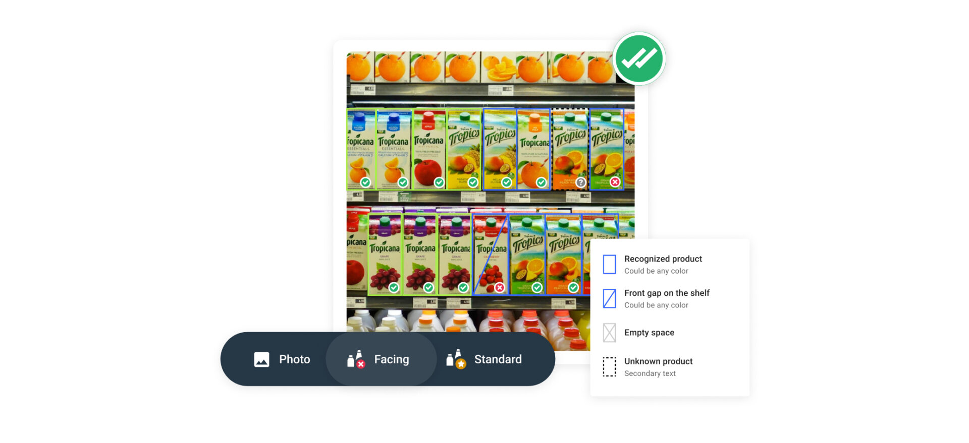
Combined with structured promotional data from TPM, it gives a more complete picture: what was planned, and what actually happened in-store.
Irregular Demand Patterns
Not all SKUs behave predictably. Some sell steadily, while others spike due to promotions, weather, or seasonality.
If these patterns aren’t captured correctly, forecasts become misleading. Especially when peaks and drops are treated as “normal” demand. Ignoring seasonality alone can reduce forecast accuracy.
Again, a proper system for Trade Promotion Management and Trade Promotion Optimization process helps with it. Not by forecasting itself, but by explaining the spikes.
When promotions are planned and recorded in a TPM/TPO system, demand peaks are no longer “unexpected.” They are linked to specific trade promotion strategies and activities: discounts, displays, and campaigns.
As a result, forecasts can separate baseline demand from promotional uplift.
Lack of Cross-Functional Collaboration
Forecasting often happens in silos: sales, marketing, and supply chain work with different assumptions.
Without shared inputs (like promo plans or expected orders), forecasts become fragmented.
A TPM/TPO solution can serve as a shared platform for several departments.
Marketing defines campaigns, sales adds expected volumes, and supply can adjust production and distribution ahead of time.
One of our clients initially adopted our TPM/TPO solution to track overall trade spend, not just promotions. But in practice, the bigger impact came from alignment.
With PromoTool, teams started working in the same environment, using the same data, assumptions, and approval flows.

High Data Volume and Complexity
Hundreds or thousands of SKUs across regions, channels, and formats create massive datasets.
Manual tools and simple models struggle to process this complexity. As a result, teams either simplify too much (losing accuracy) or spend excessive time managing data.
Just imagine a brand with 2,000 SKUs trying to forecast in Excel. Updating a single file would take hours, and errors would multiply.
New Product Launches Without Historical Data
When new SKUs have no past data to learn from, both baseline and advanced models are ineffective at the start.
Let’s say a new flavor was expected to perform like an existing SKU. However, demand turns out to be much lower, resulting in excess stock and write-offs.
How to Implement SKU-Level Demand Forecasting
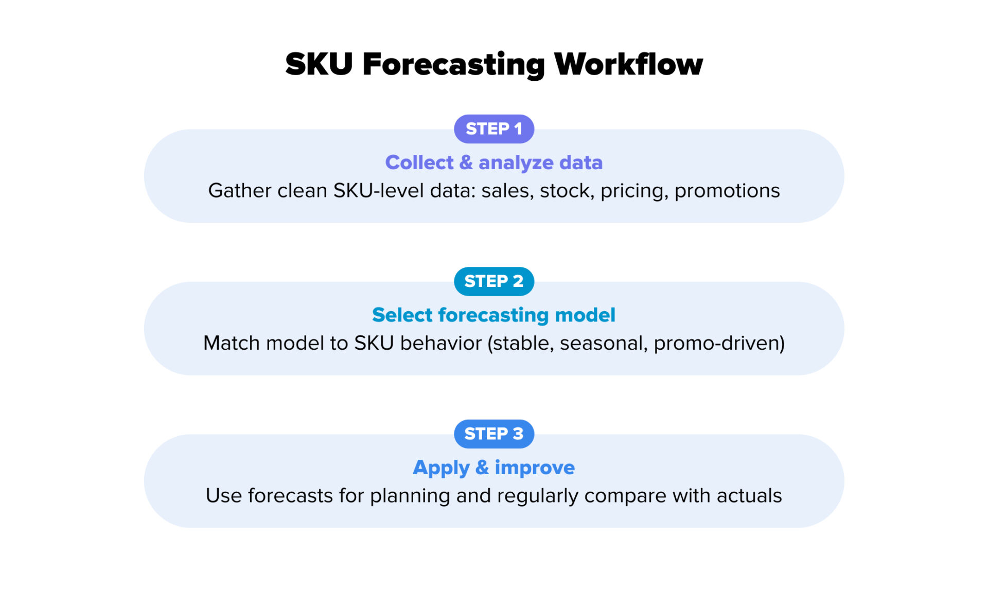
Step 1: Collect and Analyze Data
Since forecasting is data-driven, start with the basics: get your data in order.
You need sales, stock levels, pricing, and promotions. All at the SKU level. If this data is spread across files or full of gaps, the forecast won’t hold. Clean it, align formats, and make sure you’re not working with outdated numbers.
It also helps to group SKUs. For example, fast-moving products need more frequent updates than slow sellers. Treating everything the same is where many teams go wrong.
Step 2: Select the Right Forecasting Model
Some products sell steadily and are easy to predict. Others depend on seasonality or promotions and need more flexible models. In reality, most companies end up using a mix.
Trying to manage this in spreadsheets quickly becomes unmanageable. At a certain scale, tools are not optional – they’re what make SKU-level forecasting possible.
Step 3: Apply and Improve the Forecasting Process
A forecast is only useful if you act on it.
Use it to decide how much to order, when to reorder, and how much buffer stock to keep. Then check what actually happened. Did you sell more? Less? Why?
This step is ongoing. Demand changes, and your forecasts need to keep up. Teams that review and adjust regularly avoid the usual problems: stockouts of fast sellers and excess stock of slow sellers.